In the last article in this series, we introduced the core concepts of machine learning, built a single-layer neural network to learn a simple equation, and explored how TensorFlow can be used to quickly train and evaluate neural networks. With these core concepts covered, we delve into the realm of neural network-based time series forecasting, focusing on a more specific dataset. If you’re keen on hands-on learning, this article is also accessible via Google Colab.
A Primer in Time Series
Time series are ordered sequences of values equally spaced over time. Some examples could be the outside temperature taken every second for a day, the speed of a train every minute throughout a trip, or a stock price throughout time.
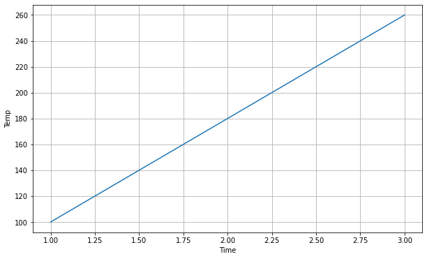
This might seem like a big jump from the data we’ve worked with thus far, but we can actually imagine our previous dataset as a time series! To visualize this, let’s plot it using matplotlib, a helpful library in Python. We can imagine x as time and y as temperature.
x = [1, 1.5, 2.0, 2.5, 3.0]
y = [100, 140, 180, 220, 260]

def plot_series(time, series, format="-", start=0, end=None, label=None):
   plt.plot(time[start:end], series[start:end], format, label=label)
   plt.xlabel("Time")
   plt.ylabel("Temp")
   plt.grid(True)

plt.figure(figsize=(10,6))
plot_series(x, y)

Let’s break down some of the most common characteristics of time series: trend, seasonality, and noise. If we imagine this graph as temperature steadily increasing over time, we could say it is trending in the upward direction, as it’s “moving” consistently in a single direction.
A time series can also have seasonality, where patterns in the series repeat at predictable intervals. In the left plot below, we’ll add a seasonal pattern to the series. If you’d like to see how this was done, please refer to the Google Colab project linked above.

Unfortunately, real-life data is usually noisy. Noise introduces randomness into the series values, without a clear trend or pattern. Let’s simulate some noise on top of the previous series above.
Now that we have an idea of what time series data looks like, what problems might we solve with it using a neural network? One of the most common things a network can be used for is forecasting, in which we take in previous values of the time series, and predict what the next values will be. We’ll start by building a naive time series forecasting model without machine learning, and then see how our neural network model compares against it.
A Naive Forecasting Model
In order to evaluate our forecasting accuracy, we’ll need to compare our predicted values against the true values in the time series. To measure our time series forecasting model’s performance, we’ll split our data into 2 periods: a training period and a validation period. As before, we’ll train our model on the training set, and then evaluate it on the validation set, updating our model’s parameters to perform better on the validation data. In addition to testing against our validation data, we can also forecast a trained model into the future, which is sometimes called the test period.
To begin, let’s split our time series into training and validation periods. We want to ensure that the consistent seasonality we see in the data is present in both the training and validation sets, so that our trained model will know what it’s looking at when the seasonality occurs in the validation set.
split_time = 1000
time_train = time[:split_time]
x_train = series[:split_time]
time_valid = time[split_time:]
x_valid = series[split_time:]

plt.figure(figsize=(10, 6))
plot_series(time_train, x_train)
plt.show()

Given that our naive model doesn’t use machine learning and requires no training, we can build and test it directly on the validation set. What might be a simple, brute-force way to predict a value at one point in time, given the values in a previous window of time? As you might guess, we’ll call this set of previous values the window, and call the number of these values the window size. Our feature data is then the values within this window, while our labeled data is the next value directly after the window, which we’ll continue to predict as we move across the time series.
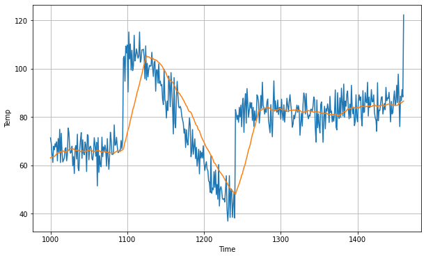
The naive model we’ll build is called a moving average model, in which we predict that the next value of the time series is the average of a set window of previous values. Let’s define our model with a window size of 30, and plot it against the validation data.
def moving_average_forecast(series, window_size):
 forecast = []
 for time in range(len(series) - window_size):
   forecast.append(series[time:time + window_size].mean())
 return np.array(forecast)

moving_avg = moving_average_forecast(series, 30)[split_time - 30:]

plt.figure(figsize=(10, 6))
plot_series(time_valid, x_valid)
plot_series(time_valid, moving_avg)

As you can see, our moving average model does a decent job of following our data, but it’s consistently lagging behind the true values after a large fluctuation. To evaluate our model, we can use the same loss function as earlier, mean squared error (MSE), and also a new loss function, mean absolute error (MAE). In MAE, the loss linearly increases as our prediction gets worse, so predictions that are especially inaccurate aren’t especially penalized like they are in MSE. Let’s see how our naive model scored.
print(keras.metrics.mean_squared_error(x_valid, moving_avg).numpy())
print(keras.metrics.mean_absolute_error(x_valid, moving_avg).numpy())
106.67456651431165
7.142418570620879
We scored an MSE of a bit over 106, and an MAE a bit over 7. Now, let’s build a model using neural networks and see how it compares!
A Neural Network Forecasting Model
As mentioned, we can now view our feature data as the windowed data values, and the labels as the next value after each window. Using the tf.data.Dataset API, we can easily construct the dataset for our network. We’ll feed our neural network windows of data to train on, as opposed to the single values in our last article’s neural network. We will also shuffle our data before training, so that our network can avoid sequence bias, where the sequence of windowed data we feed our network impacts the way it’s trained. Let’s get an idea of what the feature and label data will look like with this simple example, where the time series simply trends up from 0 to 9.
dataset = tf.data.Dataset.range(10)
dataset = dataset.window(5, shift=1, drop_remainder=True)
dataset = dataset.flat_map(lambda window: window.batch(5))
dataset = dataset.map(lambda window: (window[:-1], window[-1:]))
dataset = dataset.shuffle(buffer_size=10)
for x,y in dataset:
 print(x.numpy(), y.numpy())

[2 3 4 5] [6]
[3 4 5 6] [7]
[4 5 6 7] [8]
[1 2 3 4] [5]
[0 1 2 3] [4]
[5 6 7 8] [9]
Now that we have a visual idea of how our data will be fed in, we can prepare the true dataset for our neural network. We’ll use the same training and test data as our naive model, and format it into our feature windows and label values.
window_size = 30
batch_size = 32
shuffle_buffer_size = 1000

def windowed_dataset(series, window_size, batch_size, shuffle_buffer):
 dataset = tf.data.Dataset.from_tensor_slices(series)
 dataset = dataset.window(window_size + 1, shift=1, drop_remainder=True)
 ...
 return dataset

dataset = windowed_dataset(x_train, window_size, batch_size, shuffle_buffer_size)
Next, we’ll define our neural network much like we did in our last article. We’re feeding in windows of 30 data values, so the input shape of our model is 30. We’ll define our single layer separately, so that we can later inspect the layer’s weight values. We again set our loss function to Mean Squared Error, and our optimizer to Stochastic Gradient Descent, and train it for 100 epochs.
layer = tf.keras.layers.Dense(units=1, input_shape=[window_size])
model = tf.keras.models.Sequential([layer])

model.compile(loss="mean_squared_error", optimizer=tf.keras.optimizers.SGD(learning_rate=1e-6, momentum=0.9))
model.fit(dataset,epochs=100,verbose=0)
Now that our model is trained, we can actually take a look at our layer weights! As you may recall, these weights are assigned to each edge in our network, and we multiply each input value by its respective weight. We then sum these values to get the value of our single hidden neuron. In our time series context, this means that we multiply the first window value by the first weight, and so on until the 30th window value. Additionally, the final value we return here is our bias, which is always added to our single neuron to get the final output value.
print("Layer weights {}".format(layer.get_weights()))

Layer weights [array([[ 0.027791  ],
       [-0.03986489],
       [ 0.0099981 ],
       …,
       [ 0.44601417]], dtype=float32), array([0.01506113], dtype=float32)]
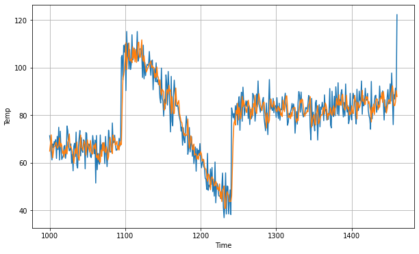
Now that we’ve trained our model, let’s see how it performs! We iterate through the validation set, and plot the network’s predictions against the true values.
forecast = []

for time in range(len(series) - window_size):
 forecast.append(model.predict(series[time:time + window_size][np.newaxis]))

forecast = forecast[split_time-window_size:]
results = np.array(forecast)[:, 0, 0]

plt.figure(figsize=(10, 6))
plot_series(time_valid, x_valid)
plot_series(time_valid, results)

Just as with our naive model, we can now take a look at our model’s accuracy using the MSE and MAE metrics.
print(keras.metrics.mean_squared_error(x_valid, results).numpy())
print(tf.keras.metrics.mean_absolute_error(x_valid, results).numpy())
45.665363
5.0795245
Our mean squared error has decreased by more than 60, while our mean absolute error has decreased by more than 2! This is a significant improvement over the naive model, and this was only using a single hidden neuron in a single layer!
In this article, we covered how time series data can be broken down into the characteristics of trend, seasonality, and noise, and how a machine learning model can learn to recognize these trends and seasonal patterns in the data. We saw how to label our data for training using windows, and how this windowed data technique can be used to build a simple moving average model. We then saw how to shuffle our training data to avoid sequence bias when training a neural network, and how this network approach significantly improved our time series forecasting accuracy.
If you’ve ever heard the term deep learning, this involves building networks with multiple hidden layers, and using a variety of other tools to build more sophisticated and accurate models. With TensorFlow, updating our model to a Deep Neural Network (DNN) is very simple. In the next article, we’ll learn to build and fine-tune a DNN to more accurately forecast our time series, and see how it can predict into the future, or test period, using real data.
About Mission Data
We’re designers, engineers, and strategists building innovative digital products that transform the way companies do business. Learn more: https://www.missiondata.com.


